Warum zufällige Kugeln immer eine Glockenkurve ergeben
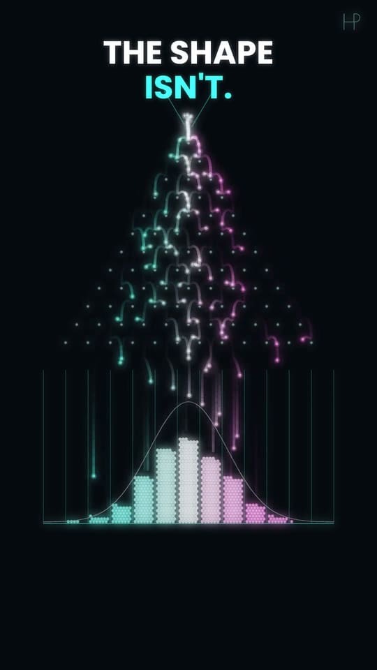
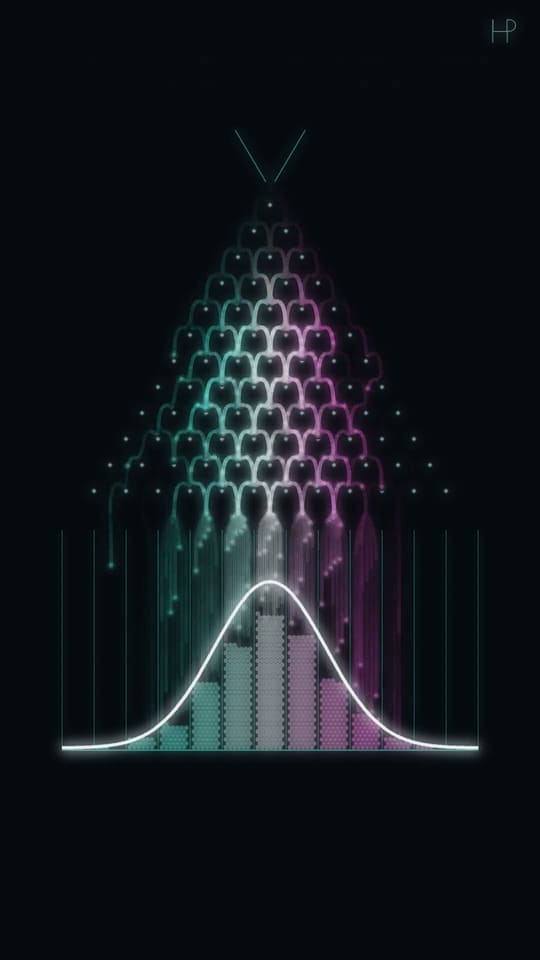
Jede Kugel springt zufällig nach links oder rechts. Tausende von ihnen zeichnen trotzdem dieselbe Glockenkurve.
Läuft nach einem Klick von YouTube.
Probier es aus: Ändere die Regel
Wirf ein paar Kugeln ein. Die weiße Kurve zeigt, wo sie sich sammeln sollten.
Warum es funktioniert
An jedem Stift springt eine Kugel zufällig nach links oder rechts. Eine Kugel verrät nichts, aber Tausende häufen sich jedes Mal zur selben Glockenform, weil es viel mehr Wege in die Mitte gibt als an die Ränder.
P(k) = C(n, k) · pᵏ · (1 − p)ⁿ⁻ᵏMitte = n·pBreite = √(n·p·(1 − p))
Bau es selbst
Python 3 · numpy · matplotlib5000 Kugeln durch 12 Reihen, ihre Fächer im Vergleich mit der Binomialkurve.
"""Galton board: every ball goes left or right at random at each of 12 rows of pegs.
Run: python galton-board.py   (needs: pip install numpy matplotlib)
"""
from math import comb

import numpy as np
import matplotlib.pyplot as plt

plt.style.use("dark_background")

rows, balls, p = 12, 5000, 0.5  # p: the chance of bouncing right
rng = np.random.default_rng()

bins = (rng.random((balls, rows)) < p).sum(axis=1)  # a ball's bin = how often it went right
counts = np.bincount(bins, minlength=rows + 1)

k = np.arange(rows + 1)
expected = [balls * comb(rows, i) * p**i * (1 - p) ** (rows - i) for i in k]  # the binomial curve

plt.figure(figsize=(7, 4))
plt.bar(k, counts, color="#5eead4", label="balls")
plt.xlabel("bin = times the ball went right")
plt.plot(k, expected, color="white", label="C(n, k) p^k (1-p)^(n-k)")
plt.legend()
plt.show()

# Try: p = 0.65 tilts the board; rows = 24 makes the bell narrower for its width
Probier: Setze p = 0.65, um das Brett zu kippen, oder rows = 24: Die Glocke wandert, dann wird sie schmaler.
Lerne dieses Skript Zeile für Zeile, mit Übungen und einem Quiz → · starte es in Google Colab (auf Englisch) →
Für Lehrkräfte: ein Stundenentwurf für 45 Minuten und ein Arbeitsblatt auf drei Niveaus →
Die Mathematik, wie der Film sie erzählt
Die Notizen zum Film lesen (von YouTube, auf Englisch)
At each peg a ball goes left or right with equal chance, independently of everything before. After 12 rows its bin is simply the number of times it went right — 12 coin flips. There is exactly one route to the far-left bin (left, left, left… twelve times) out of 4,096 possible routes, but 924 different routes to the centre bin (any six lefts and six rights).
More routes means more balls, and the route counts are the numbers of Pascal's triangle: 1, 12, 66, 220, 495, 792, 924… Plotted, they form the binomial distribution, which for many flips becomes the normal "bell" curve — de Moivre found this in 1733, and Francis Galton built this board in 1876 to show it. In the second act every peg is rigged to send 65% of balls right: the bell does not break, it just moves to 12 × 0.65 = 7.8. In the third act each ball flips 24 coins instead of 12: relative to the board, the bell gets narrower, because the spread grows only with the square root of the number of flips.
The white curve is drawn before the balls arrive; every ball's route is a genuine random draw, and the run shown is one take chosen for how cleanly it fills the curve.
Colour is route: balls that went left more than expected are teal, right more than expected pink, right on target white.
Aus der Beschreibung von Random Balls Build a Perfect Bell Curve (auf Englisch).