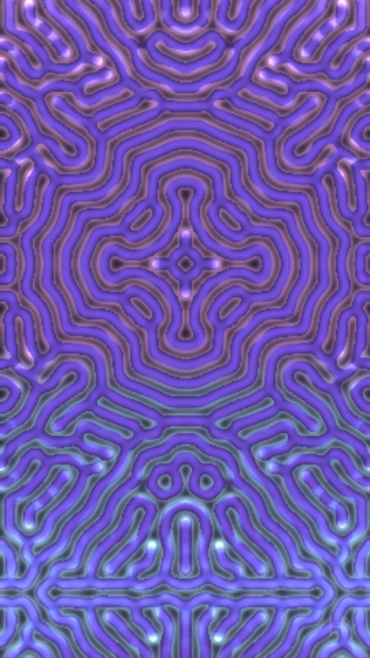
Wie zwei Chemikalien Flecken und Streifen wachsen lassen
Zwei Chemikalien: Die eine nährt, die andere breitet sich aus. Flecken und Streifen wie auf der Haut von Tieren wachsen von selbst.
Läuft nach einem Klick von YouTube.
Probier es aus: Ändere die Regel
Schritte: 0. Tippe auf die Schale, um einen Tropfen B hinzuzufügen. Dieselben zwei Gleichungen ergeben jede Voreinstellung; nur f und k ändern sich.
Warum es funktioniert
Zwei Chemikalien teilen sich eine Schale. Die eine ist Nahrung, die andere frisst sie, um mehr von sich selbst zu bilden, und beide breiten sich aus. Aus einem einzigen Tropfen wächst die zweite ganz von selbst zu Flecken, Streifen oder einem Labyrinth, wie die Zeichnung auf der Haut eines Tieres.
∂A/∂t = D_A·∇²A − A·B² + f·(1 − A)∂B/∂t = D_B·∇²B + A·B² − (f + k)·B
Bau es selbst
Python 3 · numpy · matplotlibEine Schale von 128 × 128, sechs Tropfen B, 6000 Schritte der Gray–Scott-Regel.
"""Turing patterns: the Gray-Scott reaction-diffusion rule on a 128 x 128 grid.
Run: python turing-patterns.py   (needs: pip install numpy matplotlib; takes a few seconds)
"""
import numpy as np
import matplotlib.pyplot as plt

plt.style.use("dark_background")

size, steps = 128, 6000
f, k = 0.0545, 0.062  # feed and kill rates: coral
DA, DB = 1.0, 0.5  # A spreads twice as fast as B

A, B = np.ones((size, size)), np.zeros((size, size))
rng = np.random.default_rng()
for y, x in rng.integers(10, size - 18, (6, 2)):
    B[y : y + 8, x : x + 8] = 1.0  # six drops of B


def laplacian(Z):
    """Each cell against its neighbours: 0.2 for the four sides, 0.05 for the corners (Karl Sims)"""
    sides = np.roll(Z, 1, 0) + np.roll(Z, -1, 0) + np.roll(Z, 1, 1) + np.roll(Z, -1, 1)
    corners = (np.roll(np.roll(Z, 1, 0), 1, 1) + np.roll(np.roll(Z, 1, 0), -1, 1)
               + np.roll(np.roll(Z, -1, 0), 1, 1) + np.roll(np.roll(Z, -1, 0), -1, 1))
    return 0.2 * sides + 0.05 * corners - Z


for _ in range(steps):
    reaction = A * B * B  # one A and two B make three B
    A += DA * laplacian(A) - reaction + f * (1 - A)
    B += DB * laplacian(B) + reaction - (f + k) * B

plt.figure(figsize=(6, 6))
plt.imshow(B, cmap="magma", vmin=0, vmax=0.5)
plt.axis("off")
plt.show()

# Try: f, k = 0.039, 0.058 (a cell net) or 0.034, 0.063 (spots) -> the same rule, another pattern
Probier: Probier f, k = 0.039, 0.058 für ein Zellnetz oder 0.034, 0.063 für Flecken: dieselbe Regel, eine andere Art.
Lerne dieses Skript Zeile für Zeile, mit Übungen und einem Quiz → · starte es in Google Colab (auf Englisch) →
Die Mathematik, wie der Film sie erzählt
Die Notizen zum Film lesen (von YouTube, auf Englisch)
Two chemicals share a dish. A is food, fed in everywhere at a slow rate; B eats A to make more of itself (two B's plus one A give three B's) and is removed at a fixed rate. Both spread by diffusion, but A spreads twice as fast as B.
That one asymmetry is the whole secret: Alan Turing showed in 1952 that a "fast inhibitor, slow activator" pair turns a uniform dish unstable, so that the tiniest speck of B grows into a pattern with a built-in wavelength — spots, stripes, labyrinths, cells. The equations here are the Gray–Scott model, and only two numbers change during the film: the feed rate f and the kill rate k. Every "new species" you see is the same rule with those two dials moved a little: coral (f 0.029, k 0.057), solitons that split and travel (0.030, 0.060), a cell net (0.039, 0.058), turbulence (0.026, 0.051).
Colour is age: fresh growth fronts are pink-white, mature tissue violet, old regions indigo; the second seed carries a cyan tint so you can see where the two fronts meet. In the finale the dish is wiped and reseeded inside the shape of the channel's monogram — the same rule, confined — and then the walls are removed. These are the equations behind leopard spots, zebra stripes and the ridges on your fingertips.
Aus der Beschreibung von Two Chemicals Grow a Living Pattern (auf Englisch).